problem 1

Control-alt-i to open space for R code block

1+1

## [1] 2

5-4 

## [1] 1

3+4

## [1] 7

6*2

## [1] 12

2*2

## [1] 4

4/2

## [1] 2

6/2

## [1] 3

500/25

## [1] 20

(5+5)/5

## [1] 2

5+5/5

## [1] 6

problem 2

To create a variable use <- where the value on left side of arrow is the converted variable and the value on the right side of arrow is the new value given

1<-Annie
1 <- "Annie"
a <- Annie

annie <- 1
a <- annie
a

## [1] 1

annie

## [1] 1

To create a vector use <-c with brackets (numbers only need commas between while letters require quotation marks surrounding each letter)

vector <-c(1, 2, 3, 4)
vector <-c ("a", "b")



use : to list a sequence of numbers. To access "Help" quickly then type ? 

x<-c(0:10,50)
mean(x)

## [1] 8.75

x<-c(0:10, 50) x

variables

a<-1
b<-"hello world"
c<-"3"
class(a)

## [1] "numeric"

class (c)

## [1] "character"

vector<-c(1,2,3,4,5,6,5,7,6, 1000)
vector[7]

## [1] 5

vector [3:6]

## [1] 3 4 5 6

vector [c(8,8,8,8)]

## [1] 7 7 7 7

vector[vector>6]

## [1]    7 1000

vector[vector<6]

## [1] 1 2 3 4 5 5

vector[vector<=6]

## [1] 1 2 3 4 5 6 5 6

vector[vector>=6]

## [1]    6    7    6 1000

vector[vector==6]

## [1] 6 6

vector[vector!=6]

## [1]    1    2    3    4    5    5    7 1000

vector[6]<-3000
vector[1:2]<-10

class(vector)

## [1] "numeric"

vector[6]<-"j"

class(vector)

## [1] "character"

a<-c("1", "2","3")
class (a)

## [1] "character"

b<-a
class(b)

## [1] "character"

as.numeric(b)

## [1] 1 2 3

a<-"kjhkjhgkjhgkjhgkjhgkjhgkjjghkgjh"
a[1]

## [1] "kjhkjhgkjhgkjhgkjhgkjhgkjjghkgjh"

strsplit(a, split="j")

## [[1]]
##  [1] "k"    "hk"   "hgk"  "hgk"  "hgk"  "hgk"  "hgk"  ""     "ghkg" "h"

strsplit(a,split="[,]")

## [[1]]
## [1] "kjhkjhgkjhgkjhgkjhgkjhgkjjghkgjh"

b<-strsplit(a,split = "")



first_names<-c("Annie","Danny", "Wilson")
ages<-c(36, 44, 12)
grades<-c(89, 56, 99)

everybody<-data.frame(first_names, 
                      ages, 
                      grades)
everybody$first_names

## [1] Annie  Danny  Wilson
## Levels: Annie Danny Wilson

everybody$ages[2]<-12

notes about variable types: we can store data as a matrix

My first post

2018 | 7 | 23 Last compiled: 2019-04-08

Notice that whatever you define as a top level header, automatically gets put into the table of contents bar on the left.

My second post (note the order)

2018 | 7 | 23 Last compiled: 2019-04-08

I’m writing this tutorial going from the top down. And, this is how it will be printed. So, notice the second post is second in the list. If you want your most recent post to be at the top, then make a new post starting at the top. If you want the oldest first, do, then keep adding to the bottom

Adding R stuff

So far this is just a blog where you can write in plain text and serve your writing to a webpage. One of the main purposes of this lab journal is to record your progress learning R. The reason I am asking you to use this process is because you can both make a website, and a lab journal, and learn R all in R-studio. This makes everything really convenient and in the sam place.

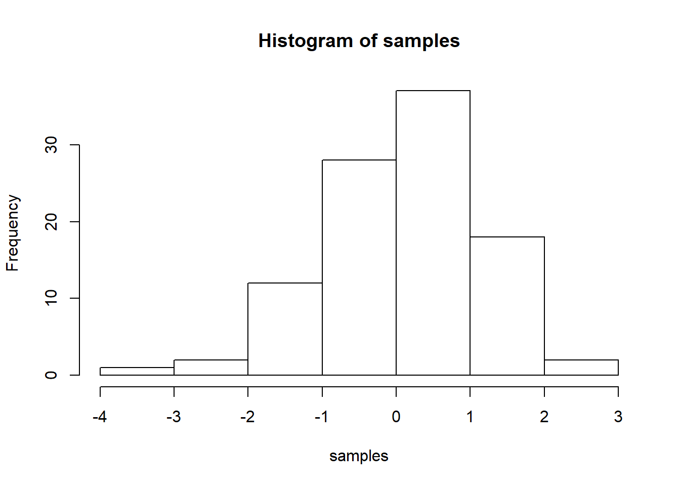
So, let’s say you are learning how to make a histogram in R. For example, maybe you want to sample 100 numbers from a normal distribution with mean = 0, and standard deviation =1, and then you want to plot a histogram. You can do this right here by using an r code block, like this:

samples <- rnorm(100, mean=0, sd=1)
hist(samples)

When you knit this R Markdown document, you will see that the histogram is printed to the page, along with the R code. This document can be set up to hide the R code in the webpage, just delete the comment (hashtag), from the cold folding option in the yaml header up top. For purposes of letting yourself see the code, and me see the code, best to keep it the way that it is. You learn all of these things and more can be customized in each R code block.

The big idea

Use this lab journal to record what you do in R. This way I will be able to see what you are doing and help you along the way. You will also be creating a repository of all the things you do. You can make posts about everything. Learning specific things in R (project unrelated), and doing things for the project that we will discuss at the beginning of the Fall semester. You can get started now by fiddling around with googling things, and trying stuff out in R. I’ve placed some helpful starting links in the links page on this website

What can you do right now by yourself?

It’s hard to learn programming when you don’t have specific problems that you are trying to solve. Everything just seems abstract.

I wrote an introductory programming book that introduces R, and gives some concrete problems for you to solve.

To get the hang of journaling and solving the problems to learn programming, my suggestion is that you use this .Rmd file to solve the problems. It would look like this:

Problem 1

Do simple math with numbers, addition, subtraction, multiplication, division

1+2

## [1] 3

2*5

## [1] 10

5/3

## [1] 1.666667

(1+6+4)/5

## [1] 2.2

Problem 2

Put numbers into variables, do simple math on the variables

a<-1
b<-2
a+b

## [1] 3

d<-c(1,2,3)
e<-c(5,6,7)
d+e

## [1]  6  8 10

d*e

## [1]  5 12 21

d/e

## [1] 0.2000000 0.3333333 0.4285714

Problem 3

Write code that will place the numbers 1 to 100 separately into a variable using for loop. Then, again using the seq function.

# for loop solution
# i becomes the number 1 to 100 at each step of the loop


a <- length(100) # make empty variable, set length to 100
for (i in 1:100){
  a[i] <-i #assigns the number in i, to the ith index of a
}

print(a)

##   [1]   1   2   3   4   5   6   7   8   9  10  11  12  13  14  15  16  17
##  [18]  18  19  20  21  22  23  24  25  26  27  28  29  30  31  32  33  34
##  [35]  35  36  37  38  39  40  41  42  43  44  45  46  47  48  49  50  51
##  [52]  52  53  54  55  56  57  58  59  60  61  62  63  64  65  66  67  68
##  [69]  69  70  71  72  73  74  75  76  77  78  79  80  81  82  83  84  85
##  [86]  86  87  88  89  90  91  92  93  94  95  96  97  98  99 100

# for loop solution #2

a<-c() #create empty variable using combine command
for (i in 1:100){
  a<-c(a,i) # keeps combining a with itself and the new number in i
}
print(a)

##   [1]   1   2   3   4   5   6   7   8   9  10  11  12  13  14  15  16  17
##  [18]  18  19  20  21  22  23  24  25  26  27  28  29  30  31  32  33  34
##  [35]  35  36  37  38  39  40  41  42  43  44  45  46  47  48  49  50  51
##  [52]  52  53  54  55  56  57  58  59  60  61  62  63  64  65  66  67  68
##  [69]  69  70  71  72  73  74  75  76  77  78  79  80  81  82  83  84  85
##  [86]  86  87  88  89  90  91  92  93  94  95  96  97  98  99 100

# seq solution
a <- seq(1,100,1) # look up help for seq using ?seq() in console
print(a)

##   [1]   1   2   3   4   5   6   7   8   9  10  11  12  13  14  15  16  17
##  [18]  18  19  20  21  22  23  24  25  26  27  28  29  30  31  32  33  34
##  [35]  35  36  37  38  39  40  41  42  43  44  45  46  47  48  49  50  51
##  [52]  52  53  54  55  56  57  58  59  60  61  62  63  64  65  66  67  68
##  [69]  69  70  71  72  73  74  75  76  77  78  79  80  81  82  83  84  85
##  [86]  86  87  88  89  90  91  92  93  94  95  96  97  98  99 100

<<<<<<< HEAD # Loading an R package

What is an R package? R base functions are under “packages” tab. It’s a library of functions.

To locate existing package: Packages->Install-type the package you want->click install

Important: you must turn on functions in order to use them in a package. You must first load the package. You can do that by clicking on package from the library OR you can put ‘library(ggplot2)’ for example to have it highlighted/selected.

my_function<-function(input){
#body of code
return (output)
}

Write a function

add_one<-fuunction(x){ return(x+1) }

Another approach: #add one to x, and save output

add_one<-function(x){

save_result<-x+1

return(save_result)

add_one(2)
}

output the contents of save_result

Another approach:

add_one<-function(x)return(x+1)

No input function example: “Roll the dice”

` Let’s try again:

roll_dice<-function(){
  return(sample(1:6,1))
}

sample(1:6,1)

## [1] 1

roll_dice<-function(){
return(sample(1:6,1))
}

Let’s say we have a bunch of numbers and we want to put it into a function. #declare a function

my_sum<-function(x){
get_sum<-sum(x)
}

my_sum<-function(x){
 get_sum<-sum(x)
  print("world")
 return("hello")
}

my_sum<- function(x){
  get_sum<- sum(x)
  print("world")
  return("hello")
}


a<-c(1,2,3)
my_numbers<-c(1,2,3,4,5,6)

my_sum<-function(x){
get_sum<-sum(x)
}

my_sum(my_numbers)

declare a variable

ranged_mean<- function(x, min_val, max_val){
  restricted_values<- x[x>min_val &
                        x< max_val]
                        return(mean(restricted_values))
}

some_numbers<-c(3,4,3,2,3,4,5,6,7,8,8,8,9,8)

ranged_mean(some_numbers, 2,4)

#sometimes you will have multiple lists that you want to combine

ranged_mean2 <- function(x, min_val, max_val){
  restricted_values <- x[x>min_val & 
                        x< max_val]
  
  outputs<- list(original_values = x,
        restricted_vallues = restricted_values)
        
  some_numbers<-c(3,4,3,2,3,4,5,6,7,8,8,8,9,8)

ranged_mean(some_numbers, 2,4) 
}

Practice Graphs

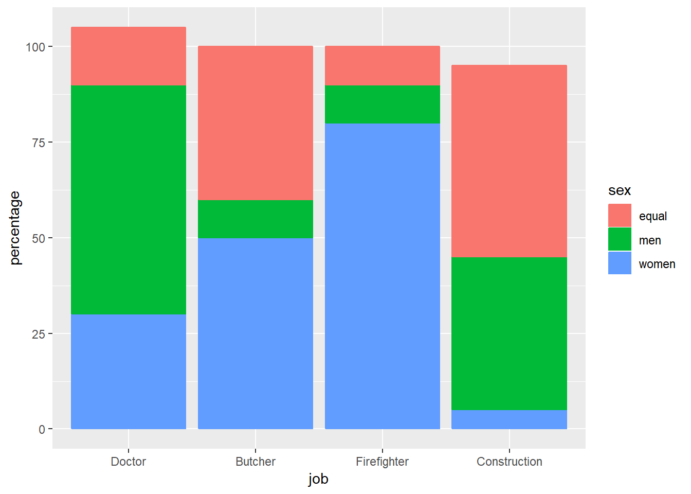
library (ggplot2)
job <- rep(as.factor(c("Doctor","Butcher","Firefighter", "Construction")),3)
levels(job)<-levels(job)[c(3,1,4,2)]#since 

sex <- as.factor(c("equal", "women", "men"))
percentage <- c(10,30,40,40,80,60,50,50,10,15,5,10)

plot_df <- data.frame(job,
                      sex,
                      percentage)

# basic bar graph

ggplot(plot_df, aes(x=job,y=percentage,
                    group=sex, #by adding group factor then you can combine 2 factors
                    color=sex,
                    fill=sex))+ #color factor refers to the border color and fill refers to entire color of the bar
  geom_bar(stat="identity") #position=dodge makes it side by side bars, without it the bars will be stacked